Arrays

What is an Array?

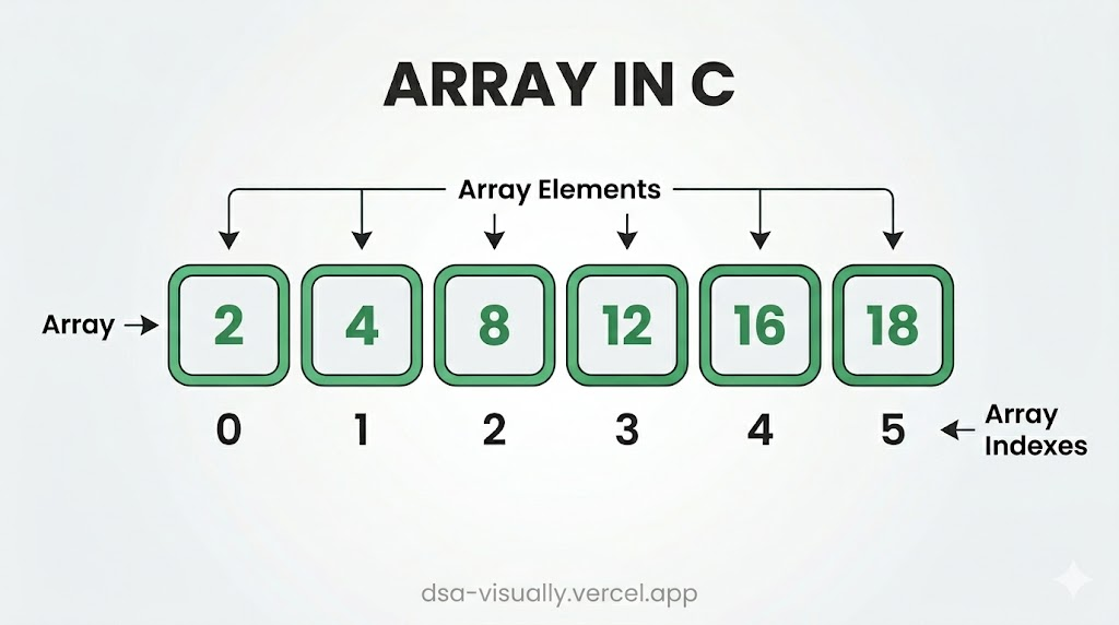
An Array is the most fundamental and widely-used data structure in computer science. It stores a fixed-size, ordered collection of elements of the same data type in contiguous (adjacent) memory locations. Because every element occupies the same amount of memory, the CPU can jump to any element instantly using a simple arithmetic formula — making random access O(1).

---

Memory Layout

When you declare an array of integers, the operating system allocates a single, unbroken block of memory. Each element sits right next to the previous one:

Index:   [  0  ][  1  ][  2  ][  3  ][  4  ]
Value:   [ 10  ][ 20  ][ 30  ][ 40  ][ 50  ]
Address: [1000 ][1004 ][1008 ][1012 ][1016 ]   (4 bytes per int)

The address of any element is computed as:

address(i) = base_address + i × element_size

This is why indexing is O(1) regardless of array size — the CPU performs one multiplication and one addition.

---

Core Operations & Time Complexities

Operation	Time Complexity	Notes
Access by index	O(1)	Direct address computation
Search (unsorted)	O(N)	Must scan every element
Search (sorted)	O(log N)	Binary search possible
Insert at end	O(1) amortized	Dynamic arrays (vectors)
Insert at middle	O(N)	All right-side elements shift
Delete at end	O(1)	No shifting needed
Delete at middle	O(N)	All right-side elements shift
Traverse	O(N)	Visit each element once

Space Complexity: O(N) — proportional to the number of elements stored.

---

Types of Arrays

1. Static Arrays

Declared with a fixed size at compile time. Memory is allocated on the stack (or data segment for globals). Size cannot change at runtime.

int arr[5] = {10, 20, 30, 40, 50};  // C static array

2. Dynamic Arrays (Vectors)

Allocated on the heap and can grow or shrink at runtime. Languages like C++ (std::vector), Java (ArrayList), and Python (list) use this internally. When capacity is exceeded, the array is reallocated to roughly double its size — giving amortized O(1) push-back.

std::vector<int> v = {1, 2, 3};
v.push_back(4);  // O(1) amortized

3. Multi-Dimensional Arrays

Arrays of arrays — the most common is the 2D array used for matrices, grids, and images.

int matrix[3][3] = {
  {1, 2, 3},
  {4, 5, 6},
  {7, 8, 9}
};
// Access: matrix[row][col]  →  O(1)

---

Advantages ✅

• O(1) random access — fastest possible element retrieval.
• Cache-friendly — contiguous memory exploits CPU cache lines, giving excellent real-world performance.
• Simple and low overhead — no extra pointers or metadata per element.
• Supports binary search — when sorted, search is O(log N).
• Foundation for other structures — stacks, queues, heaps, hash tables, and strings are all built on arrays.

Disadvantages ❌

• Fixed size (static arrays) — you must know the size upfront; resizing requires copying.
• Costly insertions/deletions in the middle — O(N) shifting of elements.
• Memory waste — dynamic arrays may allocate more capacity than needed.
• Contiguous memory requirement — large arrays may fail to allocate if memory is fragmented.

---

Key Algorithmic Patterns

Mastering arrays means knowing these essential patterns:

Two Pointer Technique

Use two indices that move toward each other or in the same direction to solve problems in O(N) instead of O(N²).

Example: Finding a pair that sums to a target in a sorted array.

Sliding Window

Maintain a "window" of elements and slide it across the array, updating the result incrementally.

Example: Maximum sum subarray of size K.

Prefix Sum

Precompute cumulative sums so that any range sum query is answered in O(1).

Example: prefix[i] = arr[0] + arr[1] + ... + arr[i]
Range sum from L to R: prefix[R] - prefix[L-1]

Kadane's Algorithm

Find the maximum subarray sum in O(N) using a single pass.

maxSoFar = arr[0]
currentMax = arr[0]
for i from 1 to N-1:
    currentMax = max(arr[i], currentMax + arr[i])
    maxSoFar = max(maxSoFar, currentMax)

Binary Search on Arrays

When an array is sorted, binary search finds an element in O(log N) by repeatedly halving the search space.

---

Real-World Applications

Arrays are everywhere in software engineering:

• Image processing — a grayscale image is a 2D array of pixel intensities (0–255).
• Audio signals — digital audio is a 1D array of amplitude samples.
• Spreadsheets — rows and columns are represented as 2D arrays.
• Database engines — columnar storage uses arrays for fast scans.
• Graphics & game dev — vertex buffers, framebuffers, and tile maps are arrays.
• Machine Learning — tensors (N-dimensional arrays) are the core data unit in NumPy/PyTorch.

---

Interview Tips 💡

1. Always clarify if the array is sorted — it unlocks binary search and two-pointer approaches.
2. Ask about duplicate values — they often affect the algorithm logic.
3. Consider in-place solutions to avoid extra O(N) space.
4. For 2D arrays, think about row-major vs column-major traversal order and its cache impact.
5. Watch for off-by-one errors — use closed/open interval conventions consistently.